8 - The Toric Code (part 3)

This is part of a project to get people involved with quantum error correction. See here for more info.

I'm going to guess that no-one jumps into part 3 of something without looking at part 1 and part 2. So I'll assume you know about the toric code in this post.

Summary

We have a bunch of qubits, which we call physical qubits. These are too noisy to do anything useful. To make a useful qubit, which we call a logical qubit, we put our physical qubits on a grid.

Here the physical qubits aren't just allowed choose whether to be 0 or 1 randomly. They have to follow the rules. The rules state that every white square must have an even number of 1's around it.

We want to make it relatively hard to see whether our logical qubit value is 0 or 1. We don't want some Gremlin coming along and measuring it, because he might mess up all our quantumness. So we take the physical qubits shown in blue below. Or the ones shown in green. Or any other loop that passes through blue squares and goes through the doughnut.

We just add up all the physical qubit values along one of these loops. If the answer is odd, the logical qubit value is 1. If it is even, the logical qubit is 0.

It turns out that this measures the number of loops of 1's that pass through white squares around the torus, and tells us whether it is odd or even. The examples in (a) and (b) don't have loops like this, so they come out even. If we want our logical qubit value to be 0 we could use one of these, or a whole bunch of other possibilities. The examples in (c) and (d) have one of these loops, so they come out odd. If we want our logical qubit value to be 1 we could use one of these, or a whole bunch of other possibilities.

Errors!

How much effort would it take to mess everything up? If we've make a logical qubit with value 0, for example, how could errors make us think it was a 1?

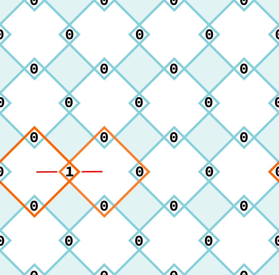
Suppose we make our logical qubit using (a), and so all physical qubits are set to 0. Then an error happens, flipping one of the physical qubits to 1. For example:

                             (e) 

Why is that red line there, you may ask. Don't worry, it'll make sense later.

For the blue physical qubits, this looks exactly the same as in (c). If we measure whether our logical qubit by looking at these, it will tell us that that its value is 1. That's wrong! All is lost!

Well, not quite yet. Remember that the 0's and 1's in the grid have to follow the rules. This error has broken them! The white squares either side of it now have an odd number of 1's around them. I have given them an orange border to shame them for their rebellion.

To make things more interesting, let's have a few more errors happen.

                               (f)

Here we have three all near each other. They form a little string of 1's. For every square, the rules are obeyed. This is because the string contributes two 1s: one when it enters and one when it leaves. But the ends of the string are a different story. These squares only get a single 1. They have an odd number of 1's. They are breaking the rules.

Correcting the errors

Finding the rule-breaking squares gives us a clue about what errors have happened. We know that they form a string, and that the orange squares are the endpoints.

That doesn't tell us exactly what happened. In both cases above, for the single error in (e) or the longer string of three in (f), the rules are broken in the same places. How can we correct the errors if we don't know what errors happened?

If errors are rare, the single error of (e) is a lot more likely than the three in (f). So we would assume that it was (e) that happened. To correct it, we would flip the corresponding physical qubit.

If we were right, and it really was (e) that happened, the 1 is flipped back to a 0. Everything is back to how it was. All the physical qubits will have the values of (a), the rules are all obeyed and our logical qubit is back to having value 0.

If we were wrong, and it was (f) that happened, we add to to the string rather than removing it. The addition joins the ends together making a loop. This is just a little loop, not one that goes around the doughnut. In fact, it is the same loop as in (b), which also corresponds to a logical qubit with value 0. We could have chosen to use these values for our physical qubits in the first place. So everything is fine. The errors have not been removed, but they have been integrated into society as productive and law abiding qubits.

In this example, it seems like the errors still leave a trace: they have added a little loop where none was before. But we can only see this because we are currently letting ourselves look at whether each qubit is 0 and 1. Actually doing these measurements would itself a source of errors. They will be outlawed in a later article, just as bit flips are here. So, in the end, the only things we'll be able to look at are whether the rules are obeyed, and what the loop around the doughnut is doing. As long as the errors don't effect these, any observable effect is completely removed.

Summary

When a bunch of bit flips happen on our nice neat code, it's best to think of them in terms of strings. When we look at the squares, and find out which ones break the rules, it tells us where the endpoints of those strings are. Then we have to try and stick the ends together and make loops.

We might not do this exactly right. We might end up making the loop bigger than it needs to be. We might end up combining a few different strings into the same loop. But that doesn't matter. All that matters is that none of the loops pass around the doughnut. As long as we achieve this, our logical qubit value will not change. The errors will have failed to have an effect.

It can be that we will get it wrong. If noise creates a string of flips that goes almost all the way around the doughnut, we'll probably end up completing it by mistake. But this needs a lot of errors to happen, and for them all to lie along the same loop. This is pretty unlikely, so we'll end up nicely correcting our errors most of the time.

What else do we need to know

We've now seen how to store a logical qubit in the toric code, and how to protect it from errors. So what else is there? Well, we've only looked at bit flip errors so far. What if those nasty gremlins were to go around measuring things that they shouldn't? They'd have to do a lot of it to cause any harm, because you can't measure the logical qubit values without looking at a whole bunch of qubits. But that's not the only trick that the toric code has up its sleeve. Next time we'll take a little look at how to foil this kind of error.

7 - The Toric Code (part 2)

This is part of a project to get people involved with quantum error correction. See here for more info.

Last time we introduced the toric code, which is a way of making many noisy qubits (which we called physical qubits) into one with hardly any noise at all (the logical qubit). We have only covered some introductory stuff so far. Today we will look at exactly how the logical qubit is stored.

For this, we again need our picture

The little squares are our physical qubits, with values either 0 or 1. For each big white square we make a measurement. This adds up all the 0's and 1's around the square and tells us only whether the result is odd or even.

In all the examples above, each square has an even number of 1's. This is because the 1's always form loops. To understand the loops in (c) and (d), we need to remember that the code is wrapped around a torus, which is the shape of a ring doughnut.

This picture (adapted from the one here) shows the kind of loop in (c) in red. Let's call this a 'loop around the doughnut'. In blue we also see a 'loop through the doughnut', which will be important soon. The purple loop is just a particularly big and fancy example of one that goes neither around nor through the doughnut.

Measuring Loops

There is obviously quite a bit difference between examples (a) and (b), and examples (c) and (d). In (c) and (d) there are loops around the doughnut, but in (a) and (b) there isn't. Is there a way we can quantify this more mathematically?

Look at the qubits shown in blue above. These are also in a loop. This loop goes through the blue squares, instead of the white ones. It also goes around the torus the other way: through the doughnut. We will use the blue qubits to make a measurement: we add up all their 0's and 1's and see if the result is odd or even.*

For example (a) we have no 1's, so the result of the measurement is obviously even. For example (b) the blue qubits will cross the small loop of 1's. They cross once when they enter and then again when they leave. This means they see two 1's. The sum of everything is then 2, so the result of the measurement is again even.

In (c) there is a loop around the doughnut, and the blue qubits will only cross it once. They see a single 1, and so the sum will be 1. The result of the measurement is odd. The same is true for (d).

This happens because of the magic of dougnuts. Usually if we have a couple of loops, either in a quantum code or in real life, they will cross each other an even number of times. Just draw a bunch of crazy overlapping loops on a piece of paper and you'll soon see it's true.

If you are drawing on a doughnut (with icing, I guess), that's not always true. When a loop round the doughnut meets one through the doughnut, they will cross an odd number of times. This is why our measurement through the doughnut didn't see the little loop of 1's in (b), but did see the big ones round the doughnut in (c) and (d).

Now we know this, we know exactly what the measurement of the blue qubits is telling us. When it says 'even', it's telling us that there's an even number of loops around the doughnut. When it says 'odd', it's telling us there is an odd number.

You probably noticed that there is a bunch of green qubits on the same picture. This is in a different place and a bit wiggly, but it still passes through blue squares and loops through the doughnut. Doing the same measurement on this will give the same results as for the blue qubits. In fact, we could use any loop through the doughnut (that passes through blue squares). They will always tell us the same information about the loops of bit flips around the doughnut (that pass through white squares).

Storing a qubit

We've been having so much fun with the toric code, we almost forgot that we need to store a logical qubit with it. This is just some information, 0 or 1, that we want to store with as few errors as possible. And we want to store it so that any quantum superposition of 0 and 1 doesn't get messed up.

For this we need to pick some sets of 0's and 1's for the physical qubits (the small squares in the toric code) that we associate with the 0 of the logical qubit, and some that we associate with the 1 of the logical qubit. For the repetition code we just picked 00000... on the physical qubits to be the logical 0, and 11111... to be logical 1 (see this post for a summary). But the toric code is a but more complicated.

In the last post we had a little wishlist of things we wanted when storing a logical qubit. One was that we shouldn't be able to measure whether it is 0 or 1 by looking at just one physical qubit.

In the toric code there is something that we cannot measure with just one physical qubit: whether there are an odd or even number of loops around the doughnut. For this we need our measurement to involve a whole bunch of physical qubits. We need enough for a loop through the doughnut, otherwise we will leave a gap. Any loops that go through the gap will mess up our measurement. So it is useless unless it goes all the way around.

For the grids drawn here we need at least four physical qubits for a loop through the doughnut. If we use bigger grids, we will need even more. The bigger the grid, the more this information gets hidden.

This is perfect for our logical qubit. If we want our logical qubit to be 0, let's use a bunch of physical qubits with an even number of loops around the doughnut. So we could set the physical bits to the values in (a) or (b), as well as loads of other possibilities. If we want our logical qubit to be 1, let's use an odd number of loops around the doughnut. We could use (c) or (d) or many others.

Now our logical bit value has been stored, and we cannot see whether it is 0 or 1 without measuring a whole bunch of physical qubits. Just as we wanted. But we have another wish to be fulfilled. We want it to be hard to turn a logical 0 into a logical 1, and vice-versa.

The toric code grants this wish too! To turn 0 into 1 we need to go from an even number of loops around the doughnut into an odd number. The only way to do this is to add one (or remove one). This means going along a loop around the doughnut and flipping every physical bit we pass.

For the grids drawn here we need to flip at least four physical bits for a loop around the doughnut. If we use bigger grids, we will need even more. The bigger the grid, the effort it takes to flip logical 0 to logical 1, and the same for 1 to 0.

The toric code grants all our wishes! It is a pretty good code for quantum information.

Correcting Errors

You may wonder if this is all quite true. You may be thinking of loopholes that could mess everything up without needing to do flips on loads of physical qubits. At the moment, loopholes do exist. But they will be closed next time when we start looking at how we can detect and correct errors.


* You might notice that this is exactly what we do when we measure the white squares. The qubits we measure in that case also form a loop that passes through blue squares. The only difference is that they are little loops, rather than big ones through the doughnut.

6 - The Toric Code (part 1)

This is part of a project to get people involved with quantum error correction. See here for more info.

We want to build a quantum computer. For that we need quantum bits or qubits. The ones we can build will always be too noisy to be used directly. We need a method to build relatively noiseless qubits out of many noisy ones. This is quantum error correction.

In this post we will start looking at one particular way to do this: the toric code. This is part of a family of codes call the surface codes, introduced over a decade ago by Alexei Kitaev. When quantum computers actually get built, it seems most likely that it will be some variant of a surface code that is doing the error correction.

Pros and Cons of the Repetition Code

Before we look at the toric code, let’s again think about the repetition code that can be used for error correction with bits (if you are new, see the last post for a summary).

In the repetition code we take many bits that are a too noisy to be useful. Let's call these physical bits. We want to use them to build one bit that is not very noisy at all, we'll call this a logical bit. We can then use logical bits to store important information, like MP3s of songs by The Wurzels.

If we want our logical bit to have value 0, we set all the physical bits to 0. If we want it to be 1, we set them all to 1. So if we use seven physical bits, we'd have

0 0 0 0 0 0 0          or          1 1 1 1 1 1 1

If noise causes some of the noisy physical bits to flip value, we end up with something like

0 0 1 1 0 0 0          or          1 1 0 0 1 1 1

To find traces of these errors we look at each pair of neighbouring physical bits, and see if their value is the same or different. It should always be the same, but strings of bit flips will have a pair that are different at each end. By finding these and pairing them up we find the errors.

We could also interpret these measurements a little differently. We can imagine that we add the two neighbouring bit values. Then we only look at whether the result is odd or even. When they are the same, the result is always even (0+0=0 and 1+1=2). When they are different, the result is always odd (0+1=1+0=1). This interpretation will help us when we make a more complicated code later in this post.

Suppose we want to flip the value stored in our logical bit. We want to flip it from 0 to 1 or vice-versa. To do this, we just flip every one of the physical bits.

0 0 0 0 0 0 0  →  1 1 1 1 1 1 1          or          1 1 1 1 1 1 1  →  0 0 0 0 0 0 0

All the bit values remain the same, so doing this leaves no trace. This is good, because it wasn't an error that did this. It was us.

Unfortunately, it is possible for errors to do this too. The probability of a bit flip error on every physical bit is very small, but it is possible. If this happens, it looks exactly like something that we might do on purpose. There is no way we could ever detect these errors. If they happen, we fail.

Obviously, we don't want to fail very often. We want the probability to be very small. This is true for the repetition code, because flipping the logical bit is not easy: It needs us to flip every physical bit. If it is hard for us, it is hard for the gremlins that cause errors too. If its hard for them, it won't happen often.

We could also use this code for qubits, using it to build a logical qubit from many noisy physical ones. It will make it rare for the logical qubit to get flipped, just as it does for logical bits.

Unfortunately, qubits suffer from another kind of noise: unwanted measurement. They are not restricted to just being 0 or 1, they can be a quantum superposition of both at the same time. If we or some gremlin look at whether our logical qubit is 0 or 1, it destroys the superpositions that we need for quantum computation. With the repetition code you can measure whether it is 0 or 1 by looking at any of the physical qubits. This makes it very likely that something will interact with them and learn the forbidden information.

So how do we protect a qubit from both types of error. We need the following two things.

• Flipping our logical bit can only be done by flipping lots of physical bits.
• It shouldn’t be possible to find out if the logical qubit is 0 or 1 by just looking at one physical qubit. Instead, finding out about the logical bit can only be done by looking at lots of physical bits.

Now let's look at a code that does this.

The Toric Code

For the toric code we don’t put our qubits in a line, we put them in a grid pattern.

This grid has lots of squares. Qubits live in the little ones, so we'll just refer to these as 'qubits'. The big white ones we will just call 'white squares'. The smaller blue ones will be 'blue squares'.

The edges of this grid are a bit odd: If you move off the top you appear at the bottom, and if you move off the right you appear at the left. The half squares on the top and bottom are actually different halves of the same square. This means that the grid is wrapped around a torus, which is a doughnut shape. It is also possible to make similar quantum codes on different surfaces. These are the surface codes.

In the repetition code we looked at whether neighbouring bits had the same or different value (or whether their sum was even or odd). We do something similar in the toric code, but not for pairs of qubits. Instead we will do it for the four qubits around each of the white squares. We add up the four bit values for each of these squares, and see whether the result is even or odd.

What patterns of bit values have all even squares? Some examples are below.

You may be wondering about the half numbers on the edges. The halves on the left will join up with the ones on the right when we wrap this around a torus. The same is true for the top and bottom.

The example labelled (a) is the easiest of all: everything is 0, so everything adds up to zero. Zero is even (don’t let anyone tell you otherwise), so all the squares are even. The one labelled (b) has a string of 1’s passing through some of the squares. When this string enters a square, we add 1 to that square’s sum. When it leaves we add another 1. As long as it leaves every square it enters, we will add two to the sum. Since two is even, the squares stay even. The only way for the string to leave every square that it enters is for it’s ends to join up, making a loop.

If you had (a) and wanted (b), all you’d need to do is flip the bits around the loop. Flipping bits around a loop always adds or removes a 1 when it enters a square, and does the same when it leaves. It doesn't matter what the original bit values are: loops of bit flips never change whether the squares are even or odd.

The two other examples have a string that stretches from left to right. This is also a loop, because the left and right edges are the same. The half squares that it passes through on left and right are just halves of the same square. In (c) we have the same bit values as (a), but with the bit values flipped on one particular line from left to right. Similarly, (d) is exactly the same as (b), except for flips on the exact same line.

The two most important things to get from all this are:

• When all squares are even, the bit values look like loops of 1’s on a background of 0’s;
• Doing bit flips around a loop doesn't change whether any square is even or odd.

Now we can start thinking about how to store information in this thing. But that’ll have to wait until next time.

The maths of qubits

This is part of a project to get people involved with quantum error correction. See here for more info.

If you are reading this, you've probably seen the word 'quantum' before. Probably in a popular science article that called it 'weird', and didn't tell you much else. Or maybe you heard it in Sci-Fi, where scientists treat equations like incantations that just need to be put it in a computer for magic to happen.

In this blog, which is usually about quantum error correction, I have been guilty of this exact same thing. But descriptions like this have serious drawbacks. They make everything seem intangible, beyond the understanding of mere mortals and only to be dealt with by great sages. This is not true at all. I work on quantum stuff, and I'm a bit of an idiot. So now it's time to tell you the truth about quantum!

To do this, we are going to need some maths. But don't be scared! Maths isn't always scary. Puzzles are maths, and they are fun (check out our own quantum game, for example).

I'm not saying that the maths in this post will be fun, but I'll keep it as simple and painless as I can. I'll only use the kind of maths that people learn at school, and I'll bear in mind that you've probably forgotten it all (and probably never understood it in the first place).

The basic maths of quantum mechanics isn’t all that hard. In fact, it can be a lot easier than what we have to deal with in the non-quantum world sometimes. If you have already been taught about vectors and complex numbers, you should probably find it quite straightforward. But for those who don't know about such things, this blog will try to give you some idea of the maths behind qubits.

States and measurements

First, let’s talk about states. We use the word ‘state’ to describe what a bit, or qubit or whatever is doing. Bits are pretty simple because they only have two possible states: 0 and 1. At any time it is either in state 0 or state 1. It cannot be both and it cannot be neither. A qubit is also built around these two basic states. But it can also be one of an infinite number of superposition states, where it is some degree of 0 and some degree of 1 at the same time.

When you measure a bit, you ask it whether it is in state 0 or state 1. You can also ask the same question of qubits. If its state is not 0 or 1, but is instead in a superposition of them, the qubit will randomly choose which one to be. If the superposition is more biased towards 0, you'll most likely get 0 and vice-versa.

It would be nice to get more information out of a qubit. It would be nice to find out exactly which of the infinite number of superposition states it is in. Unfortunately, there is no way to do this. We are limited to simply asking whether it is in one state (like 0) or a completely different state (like 1), and putting up with randomness in the result when it is neither.

Though the two basic states for a qubit are called 0 and 1, these are just labels we have chosen. They could equally be called ‘Yes’ and ‘No’, or ‘Grey’ and ‘Pineapple’, or ‘£’ and ‘%’. They are not really the actual numbers ‘0’ and ‘1’, that we can add and multiply. So it can be confusing when we start putting them into equations. To avoid this confusion, we usually write them down in a slightly strange way. For a qubit in state 0 we write |0>. For one in state 1 we write |1>. Here the | and > aren’t going to actual do anything in any equations. They are just to remind us that the 0 and 1 are names for quantum states and not actual numbers.

This notation has scared many an undergraduate physics student, so let’s avoid it here. Instead let’s use different labels for the qubit states. For the qubit state usually known as 0, let’s instead call it up. For the state usually known as 1, let’s call it down. Now that the names we are using for qubit states no longer look like numbers, we can avoid the weirdness of | and >.

Making up some maths

Now let’s try to describe quantum states with maths. One thing you need to know about maths is that it’s perfectly fine to make the rules up as you go along. This might come as a surprise to you, since you’ve probably been taught it as a set of rigid rules and methods that must be obeyed. But these are just sets of rules that turned out to be useful for something. For quantum mechanics we’ll need some new maths*, so let’s start making it up.

Firstly, it would be useful to have some way of quantifying how similar two states are. We'll call this the overlap. The states up and down are completely different, so these should have an overlap of 0. For states that are 100% the same, let's say that the overlap is 1.

Now we have a new mathematical thing to calculate. We just have to make up the mathematical rules that we can use to calculate it.

For the two states up and down, there are only four possible overlaps to calculate and we know what they should be already.

overlap of up and up = 1

overlap of up and down = 0

overlap of down and up = 0

overlap of down and down = 1

Now we need to work out overlaps for superposition states. There are many different possible superpositions of up and down, which differ by how biased they are towards one or the other. This means we need two numbers, let's call them the upness and downness, that describe how much up and down there is in a superposition

It would also be nice to have a shortened name for the superposition state that we are trying to describe. Let's just call it S. Now we need to write down the fact that S is a superposition of up and down and also what its upness and downness are, in a way that looks mathsy. How about

S = (upness of S) × up + (downness of S) × down

This nicely puts all the required information on one line. It even has has an + and some ×'s in to make it look like maths. These look suspiciously like addition and multiplication. But what does it even mean to multiply a state by a number? Or to add two states? These aren't the addition and multiplication that we are used to. I've written them in bold to help us remember that. It will turn out that they will follow similar rules to the normal ones, though. So that's why we use these symbols.

Now, what is the overlap between our superposition state S and the state up? We still haven't made up enough rules to actually calculate this, so we have to choose something. We just introduced the notion of upness, which is how much up there is in S. This seems to be pretty much the same thing as the overlap between S and up, and it wouldn't contradict any of the rules we have already if they were the same thing. So let's just make up the rule that says they are the same thing.

overlap of S and up = upness of S

There's a more complicated way we can write this, that can help us understand a little more about what is going on.

overlap of S and up = (upness of S) × (overlap of up and up)

                                         + (downness of S) × (overlap of down and up)

Here the overlap of S and up is a sum of two things. The first is the contribution from the up part of S

(upness of S) × (overlap of up and up) = (upness of S) × 1 = upness of S

This tells us that the up part of S contributes the upness (obviously), and it contributes it fully because the overlap between the up part of S and up is 1.

The second contribution is from the down part of S

(downness of S) × (overlap of down and up) = (downness of S) × 0 = 0

This tells us that the down part of S would contribute the downness if it contributed anything. But it doesn't actually contribute it because the overlap between the down part of S and up is 0.

We get a similar equation for the overlap of S and down.

overlap of S and down = (upness of S) × (overlap of up and down)

                                         + (downness of S) × (overlap of down and down)

This time the overlaps of up and down ensure that the downess contributes fully, and the upness doesn't contribute at all.

What about the overlap with something else? If we look at the overlap between S and down, and the overlap for S and up, the only difference is that one has up in and the other has down. So maybe we can just replace that with anything else too. Let's invent a new state and call it T, for no other reason but it coming after S in the alphabet. The overlap of S and T is then

overlap of S and T = (upness of S) × (overlap of up and T)

                                         + (downness of S) × (overlap of down and T)

In these equations we have × and +, multiplying and adding normal numbers. These are indeed the multiplication and addition that we are used to. From these equations you can maybe see why I used × and + before. Compare the equation for S with the equation for its overlap with T

S = (upness of S) x up + (downness of S) x down

overlap of S and T = (upness of S) × (overlap of up and T)

                                         + (downness of S) × (overlap of down and T)

These are pretty much the same. The only difference is that each state in the first one has been replaced by the overlap of that state and T in the second. This means that the second one just has normal numbers in. So the weird multiplication and addition in the first one become normal in the second. So, whatever x and + are, they must be some version of multiplication and addition that work with the states of qubits, and just become normal multiplication and addition once we just start calculating with numbers. We won't need to think much more about this, though.

Let's think more about the overlap between S and our new state T. Firstly, just like S we should be able to write T as

T = (upness of T) × up + (downness of T) × down

Earlier we made a rule that the upness of a state is the same thing as its overlap with up. This rule lets us write the equation for the overlap of S and T in a simpler way.

overlap of S and T = (upness of S) × (upness of T) + (downness of S) × (downness of T)

This lets us work out the overlap of S and T using their upness and downess, which are just numbers that we know.

Now let's ask a question for which we already know the answer. What is the overlap between S and itself? Using the maths above

overlap of S and S = (upness of S) × (upness of S) + (downness of S) × (downness of S)

= (upness of S)² + (downness of S)²

Since we are looking at the overlap between two states that are exactly the same, the answer should come out to be 1. So now we know something about the relationship between the upness and downness for any quantum superposition

upness² + downness² = 1

This makes a lot of sense. The more a state is biased towards up, the less it must be biased towards down. For example, a state with an upness of 1 (and so with an upness² of 1 too) is completely up, and so has no downness. The first concrete fact that our quantum maths has told us isn't weird at all. See, quantum mechanics isn't so strange.

Well, maybe it is a little bit strange. Note that we don't just add upness and downness here. Instead we square them first. One thing we know from school is that negative numbers square to the same value as positive ones. (-1)² = 1 just like 1² = 1, for example. So maybe this equation is telling us that its okay for the upness and downness to be negative, even though this would be a bit weird, because these numbers only need to be sensible after we've squared them. Let's keep this possibility in mind.

Left and Right

Now we've made up a nice bunch of maths, let's do something with it. Let's consider a specific superposition state, that has the same upness as downness. We can give it a name that also lies between up and down. Let's call it right.

We know that the upness and downness of right are the same, and we know that sum of their squares must be 1. With this we can get a specific number for the upness and downness: They will both be √½. Now we can write down right in our mathsy way

right = √½ × up + √½ × down,

Since we have called this right, it would be nice to know if there is a left to go with it. Is there as state that is as different from right as up is from down? If there is, we must also be able to write it down in our mathsy way

left = (upness of left) × up + (downness of left) × down

The overlap of left and right will then be, using the equation from before for S and T,

overlap of left and right = (upness of left) × (upness of right)

                                               + (downness of left) × (downness of right)

                                                    = (upness of left) × √½ + (downness of left) × √½

If left and right are to be as different as up and down, their overlap needs to be zero. This will happen only if

(downness of left) = - (upness of left)

because then we get

overlap of left and right = (upness of left) × √½ - (upness of left) × √½ = 0

So one possible choice for left is

left = √½ x up + (-√½) x down

This has an upness of √½, just as right does, but it has a downness of -√½. This is a negative downness, just like the equation earlier hinted might be possible. What does this mean? Does it make any sense? Well it is rather strange. But the equation earlier also told us to only expect the squares of numbers to be completely sensible, and (-√½)2 does give us a nice sensible ½. So let's not worry too much yet.

So far we've been thinking about everything as a superposition of up and down. But now we have left and right, which are two states just as different as up and down. What does a superposition of these look like? Something like

S = (leftness of S) × left + (rightness of S) × right

As an example, let's start with a state that has the same leftness as rightness. So

S = √½ × left + √½ × right

The overlap of this state and left is obviously √½, and the overlap for right is √½ too. What is the overlap for our trusty old friends up and down? Using the same sort of method as before, and calculating the overlaps of both left and right with up, we find

overlap of S and up = √½ × (overlap of left and up) + √½ × (overlap of right and up)

                    = √½ × √½ + √½ × √½ = ½ + ½ = 1                                

So the upness of this state is 1! Let's check the downness.

overlap of S and down = √½ × (overlap of left and down) + √½ × (overlap of right and down)

                   = √½ × √½ + √½ × (-√½) = ½ - ½ = 0                                 

It has a downness of 0! We already know a state with an upness of 1 and a downess of 0. It's up! This superposition of left and right turns out to be our good old friend up.

up = √½ × left + √½ × right

We can similarly find a superposition for down, but let's do this differently (for fun!). Let's trust that the weird × and + that we use on states really do have properties like multiplication and addition. Now let's look at the superposition

T = (-√½) × left + √½ × right

Since we have equations for left and right as superpositions of up and down, let's stick these in.

T = (-√½) × (√½ × up + (-√½) × down) + √½ × (√½ × up + √½ × down)

Doing a bunch of the maths from algebra lessons at school (see, it did come in useful), we can make this into

T = (-√½) × (√½) × up + (-√½) × (-√½) × down + √½ × √½ × up + √½ × √½ × down

= -½ × up + ½ × down + ½ × up + ½ × down                                                    

= (½ – ½) × up + (½ + ½) × down                                                                      

= down                                                                                                               

The up part disappears and the down part gets strengthened. This is exactly the sort of thing that we call an interference effect, and which causes the strange quantumness in the double slit experiment.

All states are created equal

With left and right we have another pair of states that are completely different from each other, just as different as up and down. We saw that left and right are both superpositions of up and down, but up and down can also be thought of superpositions of left and right.

This shows us an important fact about the states of quantum things, like qubits. There are no states that can claim to be the 'proper' states, with everything else just being their superpositions. Any state is as important as any other. Any state can be thought of as a superposition of other states.

This fact often gets obscured when we are talking about quantum computation. We like to think of this as a quantum version of a normal computer, so the stories we tell ourselves have to be full of 0's and 1's. But the qubit states we choose to call 0 and 1 are not really any more special than any other.

This fact also gets obscured by the intuition we get from the real world. For a cat in a box, as in Schrödingers famous thought experiment, the states 'alive' and 'dead' do seem more sensible than all the possible superposition states. This is just because big and complicated objects, like cats, are constantly interacting with other big and complicated things. These interactions, like getting looked at or and having light and the air bashing into you all the time, tend to be easier to describe using some states rather than others. When and how things bash into into you, for example, depends on where you are. So the interaction is much easier to describe using states for which you have a definite position than ones for which you are a superposition of being in different places. But for tiny things like electrons, which haven't had all the quantumness bashed out of them, superpositions of different positions are perfectly fine. And that's what we see in the double slit experiment.

Since left and right are just as important as up and down, it means we can also use them for measurements. When ask a qubit what state its in, we can ask it whether it is up or down, and a qubit in state left will have to randomly decide one or the other. But we could also ask it whether it is left or right, and an up qubit would need to randomly decide. In fact we can do an infinite number of possible measurements, where we ask if it is some state S or another state S'. The only restriction is that S and S' must always be completely different from each other: they must have an overlap of 0.

What did we just calculate?

The maths we just did involved a bunch of numbers, like overlaps and the upness and downess. But what do these numbers actually mean? Do they correspond to something that we can measure in an actual experiment, to check that our maths is actually describing qubits correctly? Fortunately, the answer is yes. And experiments have conclusively shown that we are indeed doing it right.

Basically, if we have a qubit in a state that can be written

S = (upness of S) × up + (downness of S) × down

and we measure whether it is up or down, it will randomly choose to be one or the other. The probability that it chooses up is (upness of S)². The probability of down is (downess of S)². This shows us why upness2 + downness2 = 1, as we discovered earlier. We must always get one of the two possible options, up or down. Since it is certain to get one or the other, the probability for this must be 1.

All other overlaps are similarly probabilities. If we have some state S and some other state T, the number

(overlap of S and T)² 

is the probability that you will get the result S if you are asking a qubit in state T if it is S or S'. It is also the probability that you will get the result T if you are asking a qubit in state S if it is T or T'. Here S' is the state that has no overlap with S, and T' is the state with no overlap with T. 

With this extra information we can start to wonder what it means when an overlap becomes negative. For example, say we have the state

(-1) × up

This has an upness of (-1). The condition upness2 + downness2 = 1 means that its downness must be zero, which is why it has no downness.

How does this new state differ from up? If we measure whether it is up or down, the probability of up is (-1)² = 1. So it will definitely come out to be up. If we measure anything else we will also get the same probabilities as if it were just up. The fact that its upness is (-1) rather than 1 has no effect on what we actually see in the real world. So what does a negative upness mean? Not much, it seems. The difference between any state S and the corresponding state (-1) × S is not something we can ever measure. So they are basically the same thing. Only when the difference between positive and negative happens in a superposition, as we saw for left and right, does it matter at all.
As we said before, it is the squares of the overlap that seem to have the job of being sensible. So the best way of measuring how similar two states are is to use the overlap squared, rather than the overlap itself. The overlap squared will give a value of 1 if the states are the same, 0 if they are different and something in between for something in between. It won't ever give a negative value. But the overlap itself retains the freedom be a bit crazy. It can be negative, at that lets it have some quantum fun.

What can we do now?

We now have enough maths to actually show how quantum systems can do things that would otherwise be impossible. But this post has already run on much longer than my usual 1000-1500 word limit. We probably all need to go and lie down for a week. So come back some other times and we'll look at entanglement, and how Bell's inequalities show us that it can do things more awesome than even Einstein could easily believe.

* The maths we need is called linear algebra. It’s not unique to quantum mechanics. You can use it for loads of stuff in your normal everyday life too.